Blatz-Ko Model - LS-DYNA MAT_007

Constitutive Equation

Blatz-Ko energy function implemented in lsdyna is:

\(W(\textbf{C})=\frac{G}{2}\left[I_1-3+{1\over\alpha}\left(I_3^{-\alpha}-1\right)\right]\)

where \(\bf{C}\) is the right Cauchy-Green tensor, \(G\) is the shear modulus, \(I_1\) and \(I_2\) are the first and third invariants of \(\bf{C}\) and

\(\alpha=\frac{\nu}{1-2\nu}\)

where \(\nu\) is Poisson's ratio, which is internally set to \(\nu=0.463\).

Using the above energy function, the second Piola-Kirchhoff stress is computed as

\(\begin{split}\textbf{S}&=2\frac{\partial W}{\partial \textbf{C}}=2\frac{\partial W}{\partial I_1}\textbf{I}+2\frac{\partial W}{\partial I_2}(I_1\textbf{I}-\textbf{C})+2\frac{\partial W}{\partial I_3}I_3\textbf{C}^{-1}\\&=G(\textbf{I}-I_3^{-\alpha}\textbf{C}^{-1})\end{split}\)

where \(\textbf{I}\) is unit matrix.

Cauchy stress can be obtained from the above second Piola-Kirchhoff stress.

\(\begin{split}\boldsymbol{\sigma}&=J^{-1}\textbf{FSF}^T={G\over J}[\textbf{FF}^T-I_3^{-\alpha}\textbf{F}(\textbf{F}^T\textbf{F})^{-1}\textbf{F}^T]\\&={G\over J}(\textbf{B}-I_3^{-\alpha}\textbf{I})\end{split}\)

\(\textbf{F}\) and \(\textbf{B}\) are the deformation gradient and the left Cauchy Green tensor respectively.

Parameter Identification

Blatz-Ko model in lsdyna has the only one material constant, G. So we can easily obtain it from mill sheet.

First, the principal Cauchy stress can be expressed as below.

\(\sigma_i=\lambda_i\frac{\partial W}{\partial\lambda_i}\)

\(\lambda_i\) represents stretch ratio in principal directions. This partial derivative can be solved by applying chain rule in each direction. For the first principal direction, it gives

\(\frac{\partial W}{\partial\lambda_1}=\frac{\partial W}{\partial I_1}\frac{\partial I_1}{\partial\lambda_1}+\frac{\partial W}{\partial I_3}\frac{\partial I_3}{\partial\lambda_1}\)

Assuming incompressible, \(I_3=\lambda_1^2\lambda_2^2\lambda_3^2=1\), and \(I_1=\lambda_1^2+\lambda_2^2+\lambda_3^3\). Therefore, the Cauchy stress is

\(\sigma_1=G\lambda_1^2\)

Since \(\lambda_1=\lambda\), and engineering stress, \(\sigma_\text{Eng}\) is \(\frac{\sigma_1}{\lambda}\) for uniaxial tension, this equation is written as:

\(\sigma_\text{Eng}=G\lambda\)

Finally, we can obtain G if we know the engineering stress at the stretch ratio for any material.

\(G=\frac{\sigma_\text{Eng}}{\lambda}\)

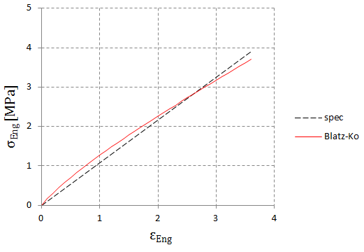
For example, if any material's tensile strength and elongation at break are 3.9MPa and 360.0% respectively, stretch ratio, \(\lambda=1+\epsilon_\text{Eng}=4.6\) and shear modulus, \(G\) is calculated from the above formula.

\(G={3.9\over 4.6}=0.85\,\text{MPa}\)

We can also get this analytical curve from the constitutive equation of Blatz-Ko model.

\(\sigma_\text{Eng}={\sigma\over\lambda}=G\left(\lambda-{1\over\lambda}\right)\)