기계공학 (Mechanical Engineering)

엑셀 차트에서 변수들의 단위가 다를 경우 보조축을 추가할 필요가 있다. 아래와 같이 Reg와 Fad 두 변수가 있을 때 Fad 변수의 보조축을 추가해 본다. 위의 변수들에 대한 분산형 차트를 만들면 아래와 같다. 그런데 하나의 세로축만 사용하면 Reg는 1 근방에, Fad는 10 근방에 분포하고 있어 추이를 가시화하기 어렵다. 따라서 Fad 변수에 대한 보조 세로축을 만든다. 먼저 Fad 계열 직선을 우 클릭하여 데이터 계열 서식을 선택한다. 데이터 계열 서식 창이 뜨면 계열 옵션에서 보조축을 선택한다. 닫기를 누르면 Fad 계열에 대한 세로축이 우측에 추가되었다.

엑셀을 사용하다 보면 하나의 셀안에 문자와 수식을 동시에 입력하고 싶을 때가 있다. 이 때는 간단히 '&' 연산자를 사용하면 된다, 아래 A1~A3 셀의 총합을 구하는 경우 하나의 셀에 단순히 결과를 넣으려면 sum 함수를 사용하면 된다(A4). 이제 A5 셀에 문자열 "Sum is "를 결과 앞에 넣고자 한다. 이 때 다음과 같이 문자열과 A4 셀의 결과값을 '&' 연산자로 묶어주면 된다. 그러면 아래와 같이 문자열과 결과치가 A5 셀에 'Sum is 6'로 표시되었다. 다음과 같이 '&' 연산자 뒤에 sum 함수를 직접 입력해도 된다.  

Training of MLP MLP learns weights and biases to minimize the difference between actual response and neural network predictions. \[{\rm H}_k^i=\sum_{j=1}^nw_j\cdot{\rm H}_{k-1}^j+\theta\cdot f_{act.}({\rm H}_k^i)\] \(w_1,\,w_2,\,\cdots,\,w_n\) : weight, θ : bias, \(f_{act.}\) : activation function Advantages - Expresses the nonlinear relationship of input and output variables well. - Able to create a meta model regardless of a lot of data. Disdvantages - User know-how dependent variables → the number of hidden layer / neuron, the activation function form. - Time consuming for training to create. Source : https://www.pidotech.com

Kriging started when Metheron mathematically established the empirical research of South African mining scientist Krige. The Kriging meta model consists of the sum of the global model f(x) and the local deviation z(x). \[y(\overrightarrow{x})=f(\overrightarrow{x})+z(\overrightarrow{x})=\sum_{i=1}^k\beta_if_i(\overrightarrow{x})+z(\overrightarrow{x})\] In the above equation, f(x) is a polynomial function, \(\beta_i\) is a regression constant vector, z(x) is a Gaussian process of a normal distribution with mean 0 and variance \(\sigma^2\), and y(x) represents the residual of the mean. In this case, the covariance in each design variable vector \({\bf x},{\bf x}'\) is as follows. \[Cov[z(\overrightarrow{x}),z(\overrightarrow{x}')]=\sigma^2R(\overrightarrow{x},\overrightarrow{x}')=\sigma^2R(\overrightarrow{d}),\ \text{where}\ \overrightarrow{d}=\overrightarrow{x}-\overrightarrow{x}'\] Where R is the correlation function. The influence of the shape of the global model an

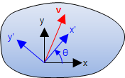
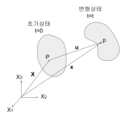
개요 (Introduction) 본 글에서는 좌표변환(coordinate transformation)을 다음 순서대로 다루게 된다: (i) 2-D 벡터 , (ii) 2-D 텐서, (iii) 3-D 벡터, (iv) 3-D 텐서, 그리고 최종적으로 4등급 텐서(4th rank tensor) 변환에 대해 알아 본다. 좌변변환의 주요 관점은, 특히 3-D에서, 변환행열(transformation matrix) 을 유도하는 것이다. 여기서는 소개만하고 변환행열 글에서 자세히 다루도록 한다. 본 글에서의 모든 좌표변환은 물체 자신은 고정된 채 좌표가 회전하는 것임을 하는 것이 매우 중요하다. 여기서 "물체"는 힘 또는 속도와 같은 벡터, 혹은 요소의 응력 이나 변형률 같은 텐서가 될 수도 있다. 물체의 회전은 회전행열 글에서 다룬다. 벡터의 2-D 좌표변환 (2-D Coordinate Transformation of Vectors) 아래와 같은 물체가 벡터를 가지고 있다고 하자. 하지만 좌표계(coordinate system)가 없이는 벡터를 기술할 방법이 없다. 그러므로 xy 좌표계가 그림과 같이 추가되면 이 벡터는 v =2 i +9 j 와 같이 기술할 수 있다. 이제 청색으로 나타낸 회전 좌표계 x'y'을 도입한다. 이 새로운 좌표계는 원좌표계로부터 반시계 방향으로 θ 만큼 회전된 것이다. 이 벡터 자신은 변한게 전혀 없다는 점에 주의한다. 하지만 새로운 좌표계에서는 다른 값으로 기술된다. 이 경우, 벡터는 새로운 y'축보다 x'축에 좀 더 평행하게 근접하므로 i ' 성분은 j ' 성분보다 클 것이다. 이 2-D 벡터 변환 방정식은 i 성분을 \(v_x\), j 성분을 \(v_y\)로 두면 \[\begin{split}&v'_x=\ \ \,v_x\cos\theta+v_y\sin\theta\\&v'_y=-v_x\sin\theta+v_y\cos\theta\end{spli

개요 (Introduction) 변형구배는 응력 을 유발시키는 변형(deformation)으로부터 병진(translation) 및 회전(rotation)의 강체 운동(rigid body motion)을 분리하는데 쓰인다. 연속체 역학(continuum mechanics)의 규약에 따라 벡터 X 는 변형전 초기 상태(undeformed reference configuration)를 그리고 x 는 변형 후 현재 상태(deformed current configuration)를 정의한다. 변형구배 (Deformation Gradient) 변형구배 F 는 변형후 x 벡터 각 성분의 초기 X 벡터 각 성분에 대한 도함수이다. x =x( X ) 로 두면 \[F_{ij}=x_{i,j}=\frac{\partial x_i}{\partial X_j}=\begin{bmatrix}\frac{\partial x_1}{\partial X_1}&\frac{\partial x_1}{\partial X_2}&\frac{\partial x_1}{\partial X_3}\\\frac{\partial x_2}{\partial X_1}&\frac{\partial x_2}{\partial X_2}&\frac{\partial x_2}{\partial X_3}\\\frac{\partial x_3}{\partial X_1}&\frac{\partial x_3}{\partial X_2}&\frac{\partial x_3}{\partial X_3}\end{bmatrix}\] 임의의 점의 변위 u 는 다음과 같이 정의할 수 있다. \[{\bf u}={\bf x}-{\bf X}\] 위의 식으로부터 x = X + u 이므로 \[{\bf F}=\frac{\partial}{\partial\bf X}({\bf X}+{\bf u})=\frac{\partial\bf X}{\partial\bf X}+\frac{\partial\bf u}{\partial\bf X}={\bf