기계공학 (Mechanical Engineering)

This article is about tips for fixing NaN errors in LS-DYNA. NaN error means the solver fails convergence for any reasons, and it was reported in d3hsp and message file. Excessive velocities due to non-physical forces and moments could act on nodes in an unstable model. First of all, by setting ISNAN=1 in *CONTROL_SOLUTION card, nodes with the out-of-range forces and moments can be reported in the message file. Identify the part(s) including the nodes by observing d3plot database in postprocessor, and check if warping elements in part itself or neighboring ones. If it is difficult to find root causes, you can reduce the d3plot interval to take a close look at them. But this could be time-consuming for a large scale model. So plot the parts internal or hourglass energies in the matsum file to check abnormal increase of them. Soft materials like rubber, foam are easy to collapse when contacting with hard materials like metal due to different modulus. After you find out the unstable pa

엑셀(Excel) 차트에는 상자그림(box plot)을 바로 그려주는 기능이 없으므로 다음 순서로 생성한다. (1) 상자그림을 만들 데이터를 입력한다. (A1~A12) (2) 각 기술통계량 을 계산한다. (통계함수는 링크를 참조) (C1~C6) (3) 그래프를 그리기 위해 아래와 같이 1사분위수를 기점으로 누적량을 계산한다. (D1~D6) D2=C3-C2, D3=C3, D4=C4-C3, D5=C5-C4, D6=C6-C5 (4) '누적량' 열 D3:D5를 데이터로 선택하여 「2차원 누적 세로 막대형」 차트를 생성한다. (5) 각 통계량 막대를 한 곳에 중첩시키기 위해 먼저 차트를 우클릭하여 「데이터 선택」을 클릭한다. (6) 「데이터 원본 선택」 창에서 「행/열 전환」을 선택하여 막대를 중첩시킨다. (7) 「축 레이블」-「편집」 버튼을 눌러 원하는 x축 레이블을 입력한다. (8) 여기서는 A1 셀을 선택하여 '데이터 1'이 표시되게 하였다. (9) 「확인」을 누르면 차트가 아래와 같이 변경된다. 최대값에 해당하는 오차 막대를 생성하기 위해 '3사분위수' 누적막대를 선택한다. (10) 「차트 도구-레이아웃-오차 막대-기타 오차 막대 옵션」을 선택한다. (11) 오차 막대 서식 창에서 「세로 오차 막대 표시 방향」으로 「양의 값」을 선택한다. (12) 원하는 「끝 스타일」을 선택한다. 여기서는 「끝 모양」을 선택하였다. (13) 오차 막대의 길이를 정하기 위해, 「오차량-사용자 지정-값 지정」을 클릭한다. (14) 윗 방향이므로 「양의 오류값」 입력란에 최대값 누적량, D6 셀을 입력한다. (15) 최소값에 해당하는 오차 막대를 생성하기 위해 '1사분위수' 누적막대를 선택한다. (16) 오차 막대 서식 창에서 「세로 오차 막대 표시 방향」으로 「음의 값」을 선택한다. (17) 원하는 「끝 스타일」을 선택한다. 여기서는 「끝 모양」을 선택하였다. (18) 오차 막대의 길이를 정하기 위해, 「오차량-사용자

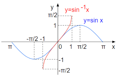
역정현함수ㆍ역여현함수 정현(sine)을 구간 \(\left[-{\pi\over 2},\,{\pi\over 2}\right]\)에서 생각하여 \(\begin{align}f(x)=\sin x,\,-{\pi\over 2}\le x\le{\pi\over 2}\end{align}\) 로 두면 \(f\)는 (1) \(\text{D}_f=\left[-{\pi\over 2},\,{\pi\over 2}\right],\,\text{R}_f=[-1, 1]\) (2) 연속 이고 강한 의미의 증가함수이다. 따라서 역함수 \(g\)가 존재하여 \(g\)는 (1) \(\text{D}_g=[-1, 1],\,\text{R}_g=\left[-{\pi\over 2},\,{\pi\over 2}\right]\) (2) 연속이고 강한 의미의 증가함수이다. 이 때 \(g\)를 \(\text{Sin}^{-1}\)로 나타내고 다음과 같이 쓴다. \(g(x)=\text{Sin}^{-1}x\) 일반으로 \(f(x)=\sin x\)에서 \(m\)을 임의의 정수라 할 때 (a) \(\text{D}_f=\left[\left(2m-{1\over 2}\right)\pi,\,\left(2m+{1\over 2}\right)\pi\right]\)라고 하면 \(\text{R}_f=[-1,\,1]\) \(f\) 는 연속이고 강한 의미의 증가함수 (b)  \(\text{D}_f=\left[\left(2m+{1\over 2}\right)\pi,\,\left(2m+{3\over 2}\right)\pi\right]\) 라고 하면 \(\text{R}_f=[-1,\,1]\) \(f\) 는 연속이고 강한 의미의 감소함수 따라서 역함수  g가 존재하여 다음과 같이 된다. (a) \(\text{D}_g=[-1, 1],\,\text{R}_g=\left[\left(2m-{1\over 2}\right)\pi, \left(2m+{1\over 2}\right)\pi\right]\) \(g\) 는 연속이고 강한 의미의 증가함수 (b) \(\tex

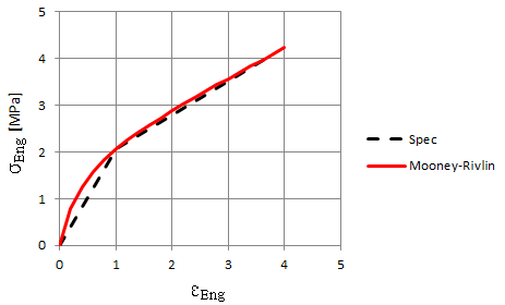
In this rubber model, the strain energy density is defined as the function of right Cauchy-Green tensor \(\textbf{C}=\textbf{F}^T\textbf{F}\), where \(\textbf{F}\) is the deformation gradient. \(W=A(I_1-3)+B(I_2-3)+C(I_3^{-2}-1)+D(I_3-1)^2\) where A, B are two material constants, and \(\begin{split}C&=0.5A+B\\D&=\frac{A(5\nu-2)+B(11\nu-5)}{2(1-2\nu)}\\\nu&=\text{Poisson's ratio}\end{split}\) \(I_1\), \(I_2\), and \(I_3\) are invariants of \(\textbf{C}\). \(\begin{split}I_1&=\lambda_1^2+\lambda_2^2+\lambda_3^2\\I_2&=\lambda_1^2\lambda_2^2+\lambda_2^2\lambda_3^2+\lambda_3^2\lambda_1^2\\I_3&=\text{det}\textbf{C}=\lambda_1^2\lambda_2^2\lambda_3^2=J^2\end{split}\) \(\lambda_1,\:\lambda_2,\:\lambda_3\) are the stretch ratio in principal directions. Parameter Identification There are two constants in this model. So we can identify them if knowing two test points in uniaxial tension. To get a useful equation, the principal stresses can be derived from strain ene

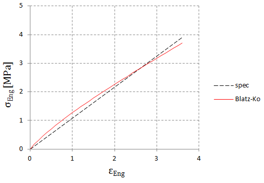
Constitutive Equation Blatz-Ko energy function implemented in lsdyna is: \(W(\textbf{C})=\frac{G}{2}\left[I_1-3+{1\over\alpha}\left(I_3^{-\alpha}-1\right)\right]\) where \(\bf{C}\) is the right Cauchy-Green tensor, \(G\) is the shear modulus, \(I_1\) and \(I_2\) are the first and third invariants of \(\bf{C}\) and \(\alpha=\frac{\nu}{1-2\nu}\) where \(\nu\) is Poisson's ratio, which is internally set to \(\nu=0.463\). Using the above energy function, the second Piola-Kirchhoff stress is computed as \(\begin{split}\textbf{S}&=2\frac{\partial W}{\partial \textbf{C}}=2\frac{\partial W}{\partial I_1}\textbf{I}+2\frac{\partial W}{\partial I_2}(I_1\textbf{I}-\textbf{C})+2\frac{\partial W}{\partial I_3}I_3\textbf{C}^{-1}\\&=G(\textbf{I}-I_3^{-\alpha}\textbf{C}^{-1})\end{split}\) where \(\textbf{I}\) is unit matrix. Cauchy stress can be obtained from the above second Piola-Kirchhoff stress. \(\begin{split}\boldsymbol{\sigma}&=J^{-1}\textbf{FSF}^T={G\over J}[\textbf{FF}^T-I_3