Mooney-Rivlin Model - LS-DYNA MAT_027

In this rubber model, the strain energy density is defined as the function of right Cauchy-Green tensor \(\textbf{C}=\textbf{F}^T\textbf{F}\), where \(\textbf{F}\) is the deformation gradient.

\(W=A(I_1-3)+B(I_2-3)+C(I_3^{-2}-1)+D(I_3-1)^2\)

where A, B are two material constants, and

\(\begin{split}C&=0.5A+B\\D&=\frac{A(5\nu-2)+B(11\nu-5)}{2(1-2\nu)}\\\nu&=\text{Poisson's ratio}\end{split}\)

\(I_1\), \(I_2\), and \(I_3\) are invariants of \(\textbf{C}\).

\(\begin{split}I_1&=\lambda_1^2+\lambda_2^2+\lambda_3^2\\I_2&=\lambda_1^2\lambda_2^2+\lambda_2^2\lambda_3^2+\lambda_3^2\lambda_1^2\\I_3&=\text{det}\textbf{C}=\lambda_1^2\lambda_2^2\lambda_3^2=J^2\end{split}\)

\(\lambda_1,\:\lambda_2,\:\lambda_3\) are the stretch ratio in principal directions.

Parameter Identification

There are two constants in this model. So we can identify them if knowing two test points in uniaxial tension. To get a useful equation, the principal stresses can be derived from strain energy function by the partial derivative as

\(\begin{split}\sigma_1&=\lambda_1\frac{\partial W}{\partial\lambda_1}\\&=\lambda_1\left(\frac{\partial W}{\partial I_1}\frac{\partial I_1}{\partial\lambda_1}+\frac{\partial W}{\partial I_2}\frac{\partial I_2}{\partial\lambda_1}+\frac{\partial W}{\partial I_3}\frac{\partial I_3}{\partial\lambda_1}\right)\\&=2\lambda_1^2A+2\lambda_1^2(\lambda_2^2+\lambda_3^2)B-4I_3^{-2}C+4I_3(I_3-1)D\end{split}\)

\(\begin{split}\sigma_3&=\lambda_3\frac{\partial W}{\partial\lambda_3}\\&=\lambda_3\left(\frac{\partial W}{\partial I_1}\frac{\partial I_1}{\partial\lambda_3}+\frac{\partial W}{\partial I_2}\frac{\partial I_2}{\partial\lambda_3}+\frac{\partial W}{\partial I_3}\frac{\partial I_3}{\partial\lambda_3}\right)\\&=2\lambda_3^2A+2\lambda_3^2(\lambda_1^2+\lambda_2^2)B-4I_3^{-2}C+4I_3(I_3-1)D\end{split}\)

To remove the Jacobian terms, \(\sigma_1\) minus \(\sigma_3\) is :

\(\begin{split}\sigma_1-\sigma_3=2(\lambda_1^2-\lambda_3^2)A+2(\lambda_1^2\lambda_2^2+\lambda_2^2\lambda_3^2)B\end{split}\)

Since \(\sigma_3=0,\;\sigma_\text{Eng}={\sigma_1\over\lambda_1}\), \(\lambda_1=\lambda\), and \(\lambda_2=\lambda_3={1\over\sqrt{\lambda}}\) in uniaxial tension by assuming incompressible, this equation is reduced :

\(\begin{split}\sigma_\text{Eng}=2A(\lambda-{1\over\lambda^2})+2B(1-{1\over\lambda^3})\end{split}\)

Now using this equation, if we know the two engineering stresses at the each stretch ratio, the two constants, A and B can be determined by performing least square fit to the two points.

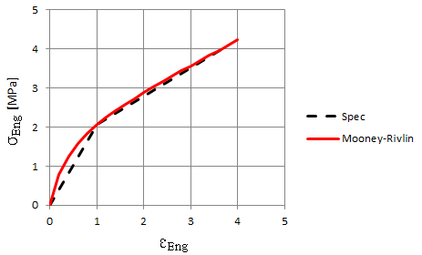
For example, a material description is obtained like the following table, then you know the engineering stresses, \(\sigma_\text{Eng}\) at 100% and 380%, break elongation respectively.

Tensile stress at 100%	2.06 MPa
Tensile stress at break	4.10 MPa
Elongation at break	380%

Using stretch ratio definition, \(\lambda=\frac{L_o+\Delta L}{L_o}=1+\epsilon_\text{Eng}\). Therefore the only unknowns are A and B with two equations. A and B can be determined for the curve to fit the two points as :

\(A=0.318,\quad B=0.540\)

Engineering stress-strain curve can be predicted from above parameters in uniaxial tension as below: