Plastic Flow Rule

Plastic flow is used to describe the plastic behavior of materials. Plastic flow theory is based on the assumption that there exist flow laws that can be used to determine the plastic deformation of a material.

The stress-strain curve above shows the plastic behavior of a typical material in uniaxial compression. The reason why compression is used instead of tension is that local necking occurs due to plastic instability in tension. On the other hand, compression does not have this phenomenon, so it can be easily converted into a true stress-true strain relationship.

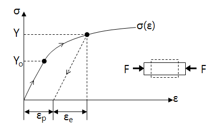
Strain can be decomposed into recoverable elastic strain, \(\epsilon_e\) and inelastic plastic strain, \(\epsilon_p\). The initial yield stress is \(Y_o\). If the elastic limit is not apparent, use the 0.2% offset yield strength, \(R_{p0.2}\). The above curve is a plastic hardening material, and as the plastic deformation increase, the yield stress also increases up to \(Y\).

The plastic flow theory for a typical unidirectional loading is developed based on the following requirement.

● The material has a linear elastic region.

● A material has an elastic limit defined as the stress, \(Y_o\) at which plastic deformation first occurs.

● Beyond this elastic limits, the stress state always exists on the yield surface. In other words, it is \(\sigma=Y\).

● Loading is defined as the stress increment, \(d\sigma\)>0. When loading occurs in the plastic region, the plastic strain increment is always \(d\epsilon_p\)>0.

● Unloading id defined as the stress increment, \(d\sigma\)<0. When unloading, the material is elastic and no additonal plastic strain is added.

● Total strain is a linear combination of elastic and plastic strain, \(d\epsilon=d\epsilon_e+d\epsilon_p\). The elastic part recovers completely, but the plastic part cannot.

● The work done by the loading-unloading cycle is either positive or zero. In other words, it is \(d\sigma d\epsilon=d\sigma(d\epsilon_e+d\epsilon_p)\)≥0. This is called the Drucker stability postulate and excludes the possibility of strain softening.

The above requirements can be expressed as a 3-dimensional stress state, and for multi-directional loadings, it is as follows.

Elasticity

When Hooke's law is applied, the relationship between stress and strain in the linear elastic range is as follows.

\[\boldsymbol\sigma={\bf C}:\boldsymbol\epsilon\]

The symbol ':' represents the inner product of tensors. Using tensor notation, it is

\[\sigma_{ij}=C_{ijkl}\epsilon_{kl}\]

Where the components of the stiffness tensor C are constants.

Yield Surface

The elastic limit is defined as the yield surface that does not depend on the plastic strain and has the following form as a function of the stress tensor, \(\boldsymbol\sigma\).

\[f(\boldsymbol\sigma)=0\]

Plastic Deformation

In strain hardening materials, the yield surface changes with the effective plastic strain, \(\epsilon_p\), and the elastic limit also changes. The change in yield surface has the form of the following equation.

\[f(\boldsymbol\sigma,\epsilon_p)=0\]

Loading

In general, a plastic load is indicated when the stress state is on the yield surface and the stress increment is directed outside the yield surface; In this case, the dot product of the stress increment, \(d\boldsymbol\sigma\), and the outer normal, \(\partial f/\partial\boldsymbol\sigma\), of the yield surface is positive.

\[d\boldsymbol\sigma:\frac{\partial f}{\partial\boldsymbol\sigma}>0\]

Neutral Loading

If the dot product of the above equation is equal to zero, it represents a neutral loading condition where the stress state moves along the yield surface.

\[d\boldsymbol\sigma:\frac{\partial f}{\partial\boldsymbol\sigma}=0\]

Unloading

In a similar way, when \(f<0\), it is unloading, and the material is in the elastic region.

\[d\boldsymbol\sigma:\frac{\partial f}{\partial\boldsymbol\sigma}<0\]

The above three loading directions can be expressed in the principal stress coordinate system as follows.

Flow Rule

In metal plasticity, the assumption that the plastic strain increment, \(d\boldsymbol\epsilon_p\), and the deviatoric stress tensor, \(\boldsymbol\sigma'\), have the same principal direction is summarized as the flow law. In other words, it is assumed that the plastic strain increment, \(d\boldsymbol\epsilon_p\), is equal to the direction perpendicular to the yield surface. That is, written in matrix and tensor notation respectively,

\[d\boldsymbol\epsilon_p=d\lambda\frac{\partial f}{\partial\boldsymbol\sigma}\qquad d\epsilon_{ij}^p=d\lambda\frac{\partial f}{\partial\sigma_{ij}}\]

Where \(d\lambda\) is the hardening parameter. Flow laws of this type are called associated flow rule, and the co-directionality assumption is called the normality condition. The yield function \(f\) is also called the plastic potential.

Consistency Condition

To complete the constitutive equation and remove the unknown variable \(d\lambda\) from the equation, the Prager consistency condition is required. Since the consistency condition is \(f(\boldsymbol\sigma,\epsilon_p)=0\), \(df=0\), so by the partial derivative of the composite function

\[df=\frac{\partial f}{\partial\boldsymbol\sigma}:d\boldsymbol\sigma+\frac{\partial f}{\partial\epsilon_p}:d\epsilon_p=0\]

Written in tensor notation,

\[df=\frac{\partial f}{\partial\sigma_{ij}}d\sigma_{ij}+\frac{\partial f}{\partial\epsilon_p}d\epsilon_p=0\]

Meanwhile, the yield function \(f\) can be written as the difference between equivalent stress, \(\overline\sigma\), and yield stress, \(Y\).

\[f=\overline\sigma-Y\]

In the patial derivative of the consistency condition, \(\partial f/\partial\epsilon_p\), the equavalent stress is independent of the effective plastic strain, so

\[\frac{\partial f}{\partial\epsilon_p}=\frac{\partial}{\partial\epsilon_p}(\overline\sigma-Y)=-\frac{\partial Y}{\partial\epsilon_p}=-h\]

Where h is the plastic modulus, which is the tangent of the hardening curvem as shown in the figure below.

Next, we consider the plastic work conjugate to obtain \(d\lambda\) from the consistency condition.

\[d\sigma_{ij}d\epsilon_{ij}^p=d\overline\sigma d\epsilon_p\]

Substituting the flow law into the above expression,

\[d\sigma_{ij}\left(d\lambda\frac{\partial f}{\partial\sigma_{ij}}\right)=d\sigma_{ij}d\lambda\frac{d}{d\sigma_{ij}}(\overline\sigma-Y)=d\lambda d\overline\sigma\]

That is, \(d\lambda=d\epsilon_p\). If we substitute the above result into the consistency condition,

\[\frac{\partial f}{\partial\sigma_{ij}}d\sigma_{ij}-hd\lambda=0\]

Now, arranging for \(d\lambda\),

\[d\lambda=\frac{\partial f}{h\partial\sigma_{ij}}d\sigma_{ij}\]

Finally, the constitutive equation can be defined by substituting the above equation into the flow law equation.

\[d\epsilon_{ij}^p=\left(\frac{\partial f}{h\partial\sigma_{kl}}d\sigma_{kl}\right)\frac{\partial f}{\partial\sigma_{ij}}\]